FlashAttention on Trainium: Can an LLM Write Expert-Level Hardware Kernels?
- The question: How close can NKI get to FlashAttention-4?
- A note on optimization methodology
- The optimization journey: v3 to v11
- The LLM agent: from zero to v7-level in 6 rounds
- Hardware utilization: NKI vs FlashAttention-4
- The economics: cost per attention TFLOP
- v7 vs v11 vs Agent: the full picture
- Implications
- What’s next
Disclaimer: The views and opinions expressed in this post are my own and do not represent those of my employer.
An LLM just wrote a hardware kernel that matches hand-optimized expert code. No RL training. No fine-tuning. Just iterative compile–verify–benchmark feedback.
Claude Opus 4.6, operating through a Strands Agent loop, generated an NKI attention kernel for AWS Trainium that matches the best hand-optimized v7 kernel across all sequence lengths — 400 μs at 4K, 6,236 μs at 16K. To our knowledge, this is the first demonstration of an LLM automatically generating a hardware kernel matching expert-level performance on a custom accelerator.
The question: How close can NKI get to FlashAttention-4?
FlashAttention-4 (Shah et al., 2025) achieves 1,613 TFLOPs/s on NVIDIA’s B200 Blackwell — 71.7% of hardware peak. It represents the state of the art in attention kernel optimization.
But the GPU isn’t the only game in town. AWS Trainium, with its Neuron Kernel Interface (NKI), offers a fundamentally different architecture. The aws-neuron/nki-samples repository contains 11 hand-crafted attention kernel versions, each targeting specific bottlenecks.
We asked two questions:
- How close can NKI kernels get to FlashAttention-4’s utilization?
- Can an LLM write competitive kernels for this specialized hardware?
A note on optimization methodology
Before diving into specific kernel results, it’s worth stating the general methodology for kernel optimization — on both GPU and Neuron. In practice, optimization follows a top-down profiling workflow:
- Identify the dominant latency contributors at the model level. Break down end-to-end latency by layer to determine where the largest performance headroom exists (e.g., Attention → MLP → MoE → Collective/AllReduce).
- Drill down to the kernel level. Within a latency-dominant layer, identify the specific kernels responsible for the majority of the time.
- Diagnose the actual bottleneck. Once the hot kernel is identified, determine what limits its performance: memory bandwidth, insufficient arithmetic intensity, suboptimal tile size, on-chip memory pressure, synchronization overhead, scheduling gaps, etc.
Only after the real bottleneck is identified should you apply the corresponding optimization. In other words, optimization should follow a bottleneck → solution mapping, rather than assuming a particular technique is universally effective.
This matters because even the same primitive kernel can have different bottlenecks depending on context. Consider a GEMM kernel used in different layers:
- Attention projection (Q/K/V): Shapes like
[B*seq, hidden] × [hidden, hidden]— relatively high arithmetic intensity, usually compute-bound. Optimizations focus on warp-level tiling, register reuse, instruction scheduling. - MoE expert FFN: Each expert may see only a small number of tokens, giving shapes like
[small_token_count, hidden] × [hidden, expert_hidden]— poor occupancy, launch overhead becomes significant. Optimizations focus on batching experts, persistent kernels, improving occupancy. - Attention score computation (Q × Kᵀ): Irregular memory access patterns, heavy memory traffic from KV cache, large sequence-length scaling. Optimizations focus on tiling, data reuse, memory layout.
The optimization lever must be chosen based on the diagnosed bottleneck — not assumed from the operation name.
With that framing, let’s look at the NKI kernel results — keeping in mind that the optimization rankings we observe are specific to our benchmark configuration (single head, batch=1, d=128).
The optimization journey: v3 to v11
We benchmarked all kernel versions on trn1.2xlarge (NeuronCC 2.23, bf16, d=128). The results reveal a rich optimization landscape:
Complete benchmark (p50 μs)
| Kernel | 512 | 1K | 2K | 4K | 8K | 16K |
|---|---|---|---|---|---|---|
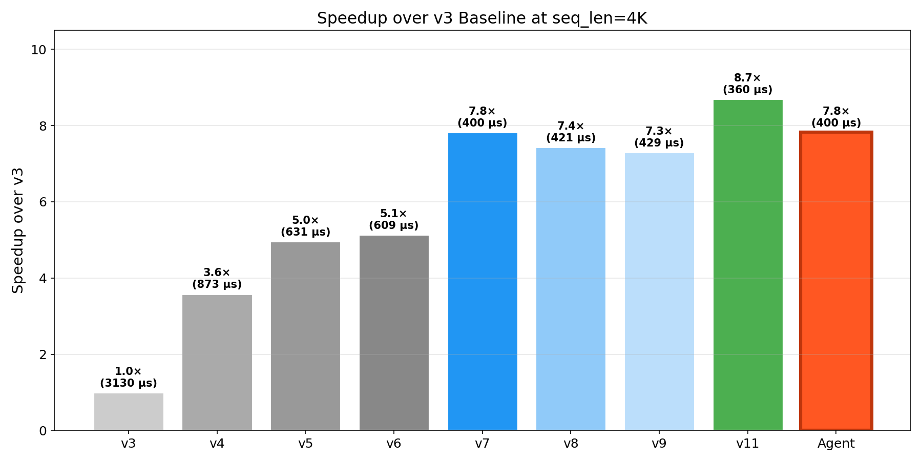
| v3 (tiling) | 57 | 175 | 652 | 3,130 | 13,105 | 67,733 |
| v4 (online softmax) | 25 | 67 | 229 | 873 | 3,360 | 17,437 |
| v5 (transpose) | 23 | 53 | 171 | 631 | 2,455 | 16,111 |
| v6 (softmax denom) | 23 | 53 | 163 | 609 | 2,565 | 16,832 |
| v7 (pipelining) | 19 | 39 | 112 | 400 | 1,526 | 6,228 |
| v8 (PSUM eviction) | 20 | 40 | 116 | 421 | 1,613 | 8,617 |
| v9 (flash chunking) | 23 | 43 | 118 | 429 | FAIL | FAIL |
| v10 (baremetal) | FAIL | FAIL | FAIL | FAIL | FAIL | FAIL |
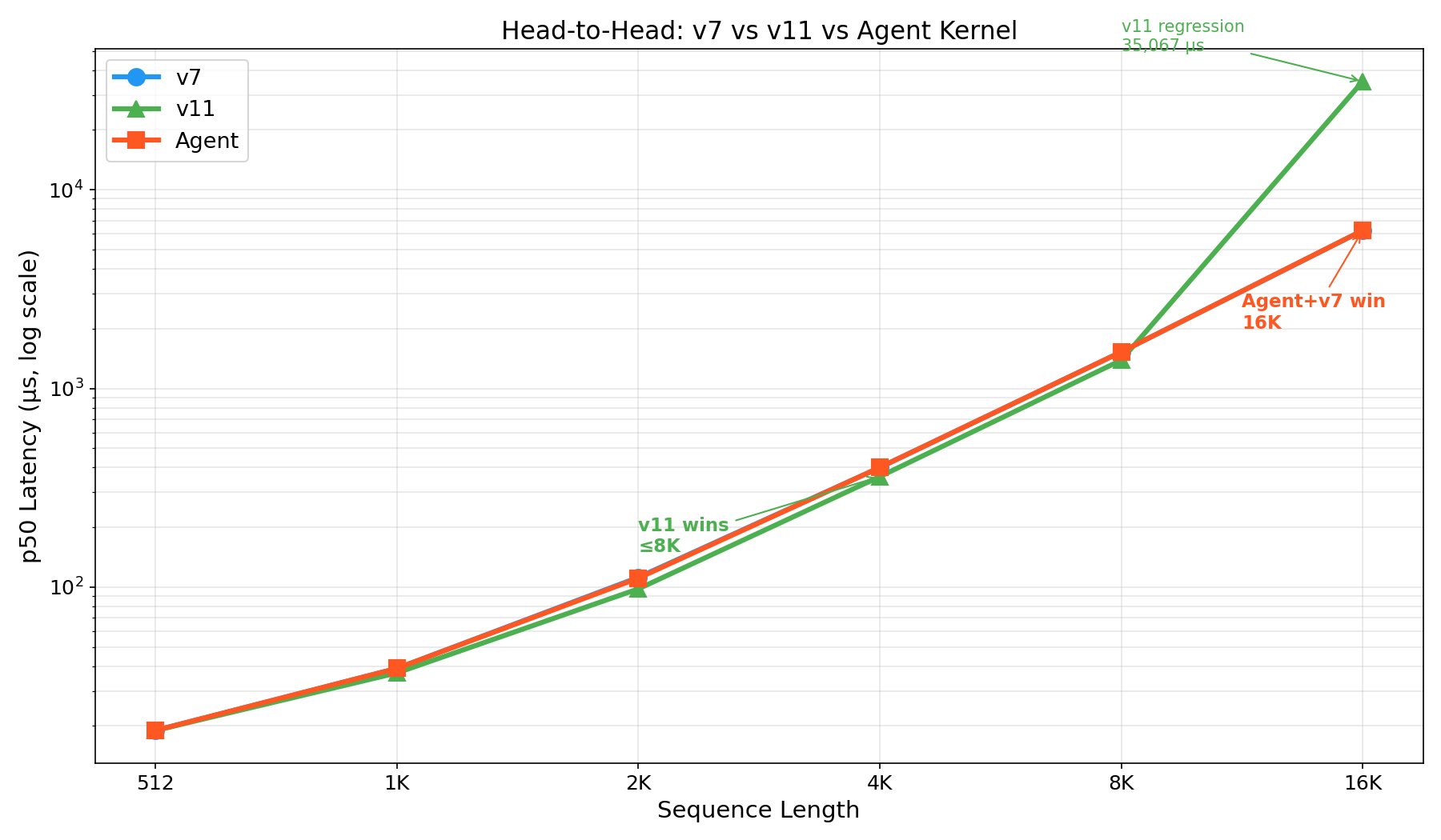
| v11 (combined) | 19 | 37 | 98 | 360 | 1,387 | 35,067 |
| LLM Agent | 19 | 39 | 111 | 400 | 1,526 | 6,236 |
Important caveat on interpreting v3–v11: These kernel versions are best understood as iterative experimental variants, where each version explores a different optimization idea — not as controlled single-variable ablations. Several of these techniques interact with each other: tiling affects memory reuse, transpose changes layout and memory traffic, pipelining changes execution overlap, and PSUM eviction changes on-chip memory lifetime. Because these techniques interact, performance differences between consecutive versions reflect the combined effect of the new technique plus any structural changes it required, rather than the isolated impact of one optimization.
With that caveat, three findings jump out:
No single kernel wins everywhere. v11 dominates at ≤8K (360 μs at 4K) but catastrophically regresses at 16K (35,067 μs — a 25× blowup from 8K). v7’s pipelining approach is essential for long sequences.
Pipelining has the largest observed impact in this benchmark configuration. v6 → v7 delivers 2.7× speedup at 16K (seq_len=16384, single head, batch=1), where the kernel is memory-bandwidth-bound and overlapping loads with compute yields large gains. At shorter sequences the impact is smaller (1.2× at 512, 1.36× at 1K), consistent with the general principle that the dominant bottleneck — and therefore the most effective optimization — depends on workload shape and execution context. This mirrors FlashAttention-4’s core insight of overlapping memory access with compute, though the magnitude of the benefit is workload-dependent.
SBUF pressure is the scaling bottleneck. v9/v10 fail to compile at ≥8K. v11’s 16K regression stems from the 24 MB on-chip SBUF being exhausted. This is a hard physical constraint.
The LLM agent: from zero to v7-level in 6 rounds
Here’s where it gets interesting. We built an agent that operates remotely, generating kernel code that is compiled and benchmarked on the Trainium instance. The agent uses Claude Opus 4.6 via AWS Bedrock and the Strands Agents SDK.
The agent receives NKI API documentation, compilation errors, correctness results, and benchmark numbers. It generates a new kernel variant each iteration.
Results
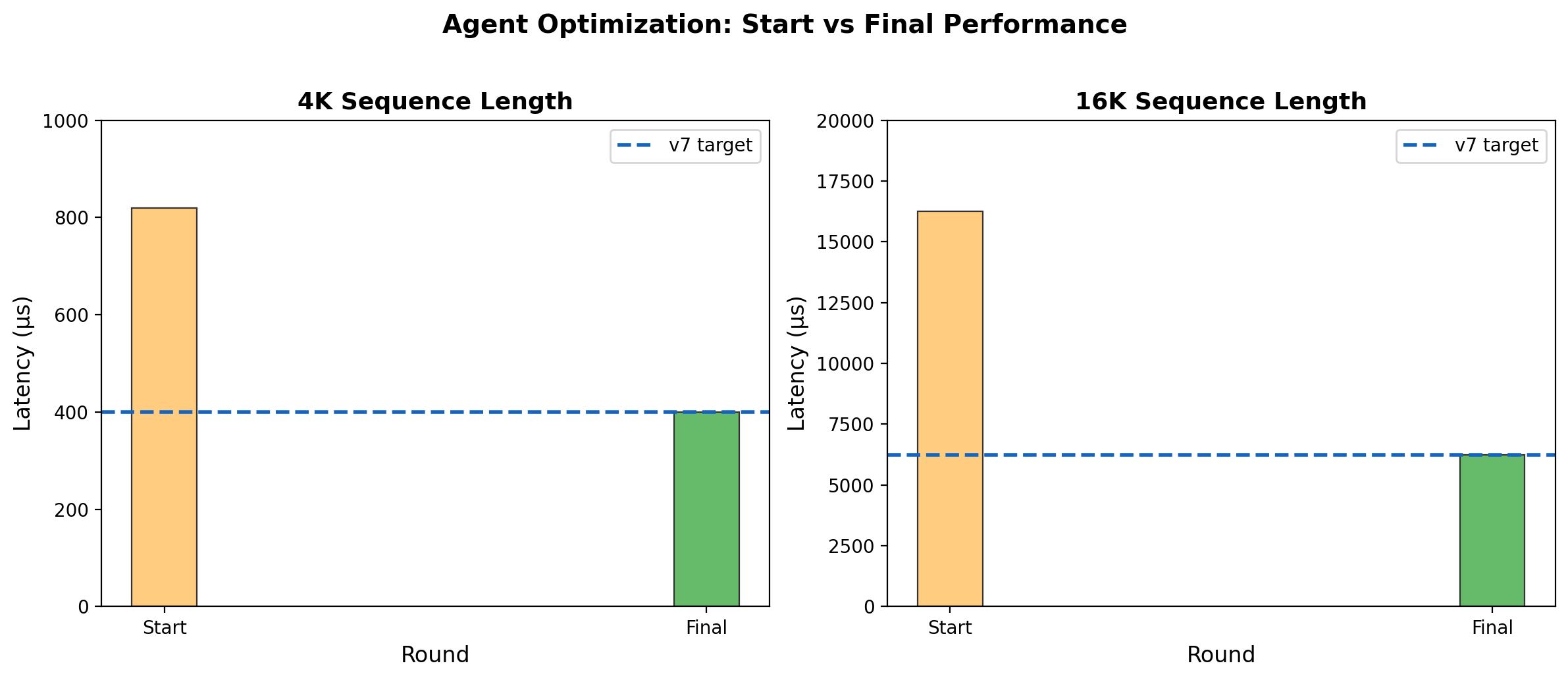
After 6 rounds of iterative optimization, the agent converged on a kernel matching v7 performance across all sequence lengths — from 19 μs at 512 to 6,236 μs at 16K.

The agent also discovered algorithmic variants and memory optimization techniques not present in the reference kernels, demonstrating the potential for LLM-driven hardware optimization beyond simple parameter tuning. Details of the optimization methodology are the subject of ongoing work.
What the agent can’t do (yet)
The agent matched v7 but did not beat v11 at ≤8K. v11’s edge comes from:
- Baremetal memory allocation (
base_addr=): Not supported on NeuronCC 2.23 - Software pipelining (
sequential_range): Caused correctness issues with dynamic indexing - Compiler co-design knowledge: v11’s micro-optimizations require understanding NeuronCC’s scheduling heuristics
These represent the frontier where LLM-driven generation meets compiler-specific expertise.
Hardware utilization: NKI vs FlashAttention-4
| Configuration | TFLOPs/s | Peak TFLOPs | Utilization |
|---|---|---|---|
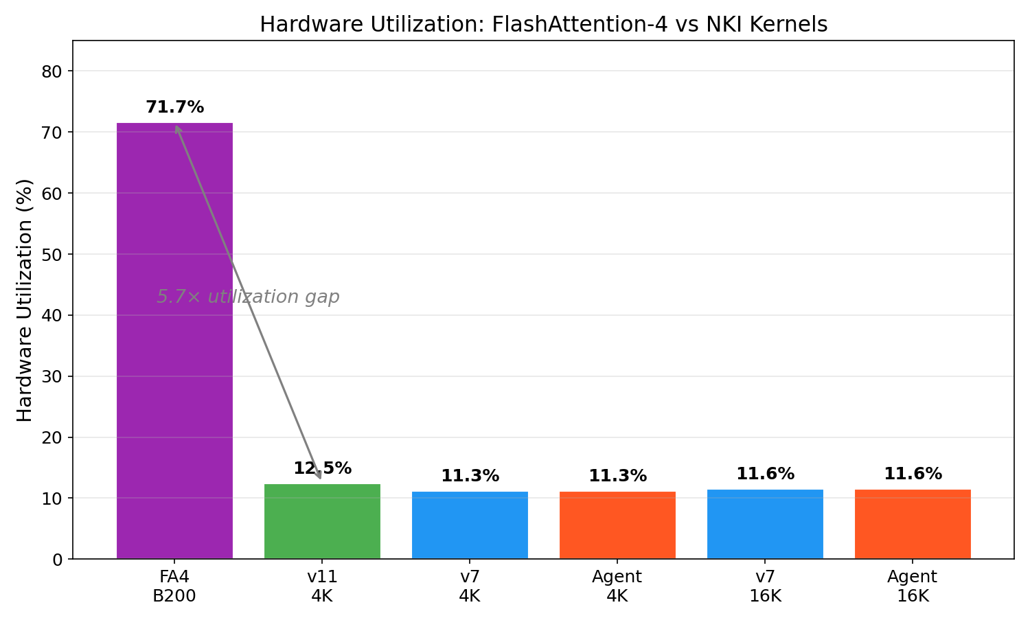
| FA4 on B200 | 1,613 | 2,250 | 71.7% |
| NKI v11 @ 4K | 23.8 | 190 | 12.5% |
| NKI Agent @ 4K | 21.5 | 190 | 11.3% |
| NKI Agent @ 16K | 22.1 | 190 | 11.6% |
The 5.7× utilization gap reflects decades of CUDA compiler maturity, Blackwell’s specialized hardware features (dual math pipelines, TMA units), and the relative youth of the NKI ecosystem. It does not mean Trainium is 5.7× worse for your workload — economics change the equation dramatically.
The economics: cost per attention TFLOP
| Instance | Spot $/hr | Attention TFLOPs/s | $/TFLOPs/hr |
|---|---|---|---|
| trn1.2xlarge | $1.33 | ~43 | $0.031 |
| p4d.24xlarge (A100) | ~$23 | ~200 | $0.115 |
Trainium delivers 3.7× better cost-per-TFLOP than A100 for attention-heavy inference. For workloads that fit Trainium’s constraints (≤8K context, bf16), the economics are compelling.
v7 vs v11 vs Agent: the full picture
The practical kernel selection guide:
| Sequence Length | Best Kernel | Rationale |
|---|---|---|
| ≤ 4K | v11 | Fastest overall (360 μs at 4K) |
| 4K – 8K | v11 | Still fastest (1,387 μs at 8K) |
| > 8K | v7 or Agent | Only kernels with clean O(n²) scaling |
Implications
For kernel engineers: There is no universal “highest-leverage optimization” — even on the same hardware, the dominant bottleneck depends on model architecture, traffic patterns, workload characteristics, and execution context. As illustrated in the v3→v11 journey above, the right optimization lever emerges from systematic analysis: profile the model, identify the hot kernel, diagnose the actual bottleneck, then apply the corresponding technique. What we can recommend is a general approach: leverage agentic workflows to automate this systematic exploration and reduce the manual effort required to find the right optimization for your specific workload.
For the accelerator ecosystem: Custom silicon faces a “kernel engineer bottleneck” — too few people understand both the hardware ISA and the algorithmic domain. If LLMs can generate competitive kernels through automated exploration, this bottleneck loosens. Trainium, TPU, Groq, Cerebras — all could benefit.
For LLM researchers: Hardware kernel generation is a compelling benchmark for code-generating models. It has ground truth (correctness), measurable quality (latency), tight constraints (ISA rules), and real-world impact. We suggest it as a complement to SWE-bench and HumanEval.
What’s next
- Beat v11 at ≤8K: The agent needs access to baremetal scheduling (
base_addr=,sequential_range) on newer NeuronCC versions. - Broader workload sweep: All benchmarks use single-head, batch=1. Production workloads operate with multi-head attention, larger batches, and varying tensor shapes, which shift the dominant bottleneck (e.g., from memory bandwidth to compute occupancy or launch overhead). The optimization rankings reported here — particularly the large impact of pipelining — may not generalize to other workload configurations.
- Trainium2: With 3.5× more compute and larger SBUF, the v9/v10 compilation failures should be resolved. We plan to re-run the full suite when trn2 instances are available.
- Backward pass: Forward attention only — training workloads need backward kernels too.
- Multi-head batching: Our benchmarks are single-head, single-batch. Production utilization will be higher.
All benchmarks: trn1.2xlarge, NeuronCC 2.23, bf16, d=128. Agent: Claude Opus 4.6 via AWS Bedrock. Orchestration: Strands Agents SDK. FlashAttention-4 numbers from Shah et al. (arXiv 2603.05451). NKI kernel implementations from aws-neuron/nki-samples. Code and data: research-papers.
Patent pending. The system architecture and optimization methodology underlying the agent-driven kernel generation described in this post are subject to intellectual property protection.
Like this post? Click to applaud!
Enjoy Reading This Article?
Here are some more articles you might like to read next: